Note: The background image is of Gilbert Strang, a great professor of Mathematics at M.I.T. His excellent book “Linear Algebra and Its Applications (third edition)” is a great book, and he has a number of excellent YouTube lectures.

Computing the Inverse in NumPy

Suppose we are given a matrix M:

.

If we had this matrix when solving a set of linear equations, M x = b, where b is a known vector, and we wish to solve for x, then solving for x is simply

x = M^-1b.

where M^-1 is the inverse of M. Using Numpy, we can easily compute the inverse:

import numpy as np
import scipy
import scipy.linalg
m1 = np.array([[0.,-3.,-2.],[1.,-4.,-2],[-3.,4.,1.]])
print(f'm1 is {m1}')
m1_inv = np.linalg.inv(m1)
print(f'm1 inverse is {m1_inv}')

And the answer is given as:

We can verify that this is the inverse by multiplying (M * M^-1) and see that it is the identity matrix.

Easy! In fact, if we take random values for the matrix M, it would work almost every time (e.g. you wouldn’t live long enough to witness one fail). The pathological case, called a singular matrix, and I will go into more detail of how to detect and potentially remediate the situation shortly. Before I talk about this failure case, let me point out that there are two broad classes of problems where you take the inverse of a matrix to get a solution:

• The class of problem where you hope for the best, if it is singular, you want to detect and report the error, but there’s no obvious fall-back strategy for getting a ‘good but not perfect’ solution, and
• The class of problems where you can still compute a reasonable value for your matrix; something that behaves like an inverse, but is well-behaved.

Singular Matrices

An example of a singular matrix, constructed specifically to make it easy to describe, is given as M_s:

You can see that it is singular, by multiplying the first row by 2, and subtracting the second row. This gives the third row. The last row, therefore, gives us no more additional information about the relative combinations of vectors and how they span the 3-dimensional space. In a 3x3 matrix, each of the column vectors define a plane. Inverting the matrix is analogous to taking the intersection point of three planes to find the point of intersection. In the singular case above, we take the intersection of two planes to find a line, but the third plane contains the entire line. In this case our matrix has a rank of 2, meaning that there are only two independent rows in the matrix.

If we attempt to compute the inverse using NumPy, as above, it will throw an exception of the type:

LinAlgError("Singular matrix")

Singular Value Decomposition

Computing the Singular Value of a matrix gives a lot of insight about the structure of a matrix.

The singular value decomposition of a matrix A, is given as:

where the columns of U and V are called the left singular vectors and right singular vectors respectively, and the diagonal matrix S is:

Computing the singular values in NumPy is easy:

u,s,vt = np.linalg.svd(m1, full_matrices=True)

All singular values s_i ≥ 0, and by convention s₁ ≥ s₂ ≥ … ≥ s_n.

Aside: Interpreting Singular Values as Incremental Approximation

Considering the column vectors u_i of U, and the row vectors v_i of V^T,

then we can see the decomposition as a sum of matrices, by taking the outer-product of the columns of U and rows of V^T

If we take n=3 then we get an exact reconstruction. The magnitude of the singular values indicates the relative importance of each term.

For example, if we consider n=1, taking only the first term, we get:

We can see that this is a fairly good approximation to the original matrix M. And using the first two terms, it is even closer.

The value here is that if we want to just keep a subset of the vectors, we can still get a good approximation, and the singular values gives us an indication of the relative importance.

Computing the Inverse with Singular Values

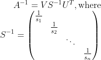
One of the interesting properties of the decomposition is that both U and V^T are orthogonal, meaning that its inverse is equal to it’s transpose.

This means that:

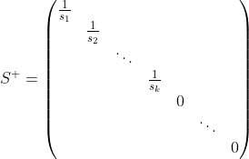
We can compute the pseudoinverse, denoted M⁺, by determining minimum thresholding criteria, of s_n that substitutes zero for sufficiently small values of 1/s_n. Taking only the first k terms, the pseudoinverse is:

In our singular case, given by M_s, the singular values, as computed by NumPy are:

6.99811874e+00 
3.32059242e+00
5.73361908e-17

The last singular value is essentially zero. Taking only the first two terms we get a pseudoinverse of the matrix. How does this help us, since it is not an actual inverse? As I will show below, for many problems, using the pseudoinverse will give you a well-behaved least-squares solution for over-determined systems.

Given the above, it is very straightforward to construct a python function that will give you a safe pseudo-inverse:

def pseudo_inverse(m, singular_value_minimum):
    # filter Si and take inverse
    ...
    inv_value = np.matmul(np.matmul(u, one_over_s), v_transpose)
    return rank,inv_value

Least Squares using Pseudo Inverse

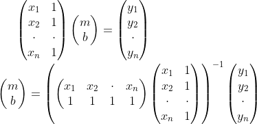
In the simple case of fitting a line in the plane to a set of data points, we seek parameters m and b, such that the line, y = mx + b, is the least squares solution.

Suppose the three points are (0,0), (2,1), and (3,3). Forming the matrix-form of the solution we get:

Solving this set of constraints using the pseudoinverse allows us to avoid the situation in which the matrix inversion would otherwise lose full rank. This might include a repetition of a point etc.

Solving this we get m = 0.92857, b = -0.21428.

Of course linear least squares is trivial, but bear in mind that we can extend this to fit tens of thousands of points in hundreds of dimensions. If any of these dimensions are degenerate, they will be omitted in the least squares solution.